Proving polynomial inequalities with sum-of-squares certificates

Thanks to Moeez Muhammad for the formalization of the key theorem required to check the certificates in Lean (see Certificate checking).

The book Semidefinite Optimization and Convex Algebraic Geometry by Blekherman, Parrilo, and Thomas is a great resource for the theory of sum-of-squares decompositions and semidefinite programming. Unless otherwise stated, all results here are from that book [1].

Overview

In this post, I will describe the workings of my new Python+Lean package for proving polynomial inequalities. Currently, support for nonlinear inequalities in Lean is limited. My package provides a Python API, a CLI, and a suite of Lean4 tactics for proving polynomial inequalities. While the software documentation is extensively covered in the README, this post will discuss the underlying theory and algorithms. The theory is based on sum-of-squares decompositions of polynomials, a powerful tool that goes back to a problem by Hilbert and its affirmative solution by Artin. The successive generalizations of this result to the so-called Positivstellensatz theorems were, in my opinion, a landmark achievement of real algebraic geometry in the 20th century. Its connection to mathematical optimization in the 21st century by Parrilo, Lassere, and others made the technique a practical computational tool.

Motivation

The current state-of-the-art

For linear inequalities, Lean already provides the linarith tactic, which works by calling the simplex algorithm. Now, as a theorem prover, Lean must prove inequalities exactly. This is fine for simplex, because it only uses the basic arithmetic operations, and it is easy to do exact arithmetic over the rationals (and so it is easy to see that a linear programming problem with rational entries yields a rational solution). Indeed, Lean contains a simplex implementation written in Lean itself. This procedure is yet treated as an untrusted oracle: it generates a (Farkas') certificate, which is then checked by the linarith tactic.

What about nonlinear inequalities? Lean4 provides the nlinarith tactic. This is really just a fancier linarith: it does some preprocessing to try to convert the problem into a linear problem, and also uses some predefined rules to add additional valid inequalities. For example, nlinarith can prove the fact that $x, y \in \mathbb{R} \implies x^2 + y^2 \geq 0$ by noting that squares are nonnegative, and then parsing this into the (linear) problem that $a, b \in \mathbb{R} \land a \geq 0 \land b \geq 0 \implies a + b \geq 0$, which is easily solved by linarith. However, nlinarith is quite limited (although sometimes the user can help it by providing additional inequalities).

The problem is hard

As I will discuss extensively in this post, an easy way to prove that a polynomial inequality like $p \geq 0$ is true is to rewrite it as a sum-of-squares of other polynomials, i.e., $p = \sum_{i=1}^k q_i^2$. Such a decomposition can be found by solving a type of optimization problem called a semidefinite program. Recall that linear inequalities can be proven using an exact implementation of the simplex algorithm. Could we use an exact algorithm for semidefinite programming to do the same thing for nonlinear inequalities? Unfortunately, the answer is less satisfying here, because algorithms for semidefinite programming do not only use the basic arithmetic operations.

The feasible set of a semidefinite program is contained inside the cone of positive semidefinite matrices, i.e., the set of matrices with all eigenvalues non-negative. In order to enforce this constraint, it is necessary to be able to compute eigenvalues, which of course is equivalent to solving for roots of a polynomial (i.e., the characteristic polynomial of the matrix). To do this exactly requires computing with algebraic numbers, which is much more difficult than computing with rational numbers (e.g., recall the Abel-Ruffini theorem that a solution in radicals may not even exist for the roots of a polynomial). All that to say: if we are trying to solve a semidefinite programming problem exactly, this requires far heavier computations with algebraic numbers, and this makes it totally intractable for all but the most trivial problems (believe me, I tried, I made an ADMM implementation in SymPy!). Expectedly, a semidefinite program with rational entries does not necessarily have rational solutions.

Why don't we use CAD?

Whenever the topic of deciding polynomial inequalities comes up, invariably the algorithm of cylindrical algebraic decomposition (CAD) also comes up, which can decide the feasibility of arbitrary Boolean combinations of polynomial inequalities. It is sound and complete, in the sense that it provides a satisfying point if it exists, and otherwise proves infeasibility. There are only a few implementations of this algorithm (see, e.g., Microsoft's Z3, or mine). So, we might be interested in whether we can take a Lean statement about polynomial inequalities, and call out to an external CAD solver.

There are some issues with this, most prominently of which is the doubly exponential time complexity of CAD, making it intractable for problems with more than a couple of variables. The other issue is in the form of answer that CAD provides, assuming the external CAD solver is used as an untrusted oracle. If it provides a satisfying point, one can simply plug it in in Lean, and, ignoring concerns about simplifying algebraic expressions, it is easy to check that the point works. However, it is far more difficult to verify that the CAD oracle has correctly determined infeasibility. CAD works by decomposing the ambient space into finitely many disjoint cells (constructed in a way that preserves certain facts about the polynomials), and then testing the polynomial inequalities over each of these cells. So, a certificate of infeasibility here would require supplying Lean with every single cell that CAD constructed, a proof that their union is the entire ambient space, and proofs that the polynomial inequalities do not hold over each cell. However, the number of cells is doubly exponential in the number of variables, making this certificate huge and difficult to check.

On the other hand, the methods I discuss here scale much better, both to run the solver and to check the certificate in Lean. As stated above, we are going to solve a semidefinite program, which is solvable in time polynomial in the size of the problem. And, when we formulate finding a sum-of-squares decomposition as a semidefinite program, the size of the semidefinite program is related to the size of the polynomial via a binomial coefficient, which, via Stirling's approximation, grows like a single exponential (contrast with the doubly exponential complexity of CAD). If our procedure determines that a system of polynomial inequalities is infeasible, it provides a small and easily checkable certificate of this fact, in sharp contrast to CAD. And, lastly, as we will see, it is often possible for the user to provide additional information in Lean which cuts down on the complexity of the problem, which fits well with the interactive nature of Lean.

Contribution

To summarize, the current support for nonlinear inequalities in Lean is limited, and while sum-of-squares is powerful, and in some ways better than CAD, the numerical nature of its solution prevents it from being used as a rigorous proof. In this post and the associated software, I implement methods that can:

Sum-of-squares decompositions

Setup

Fix a positive integer $n$ as the number of variables and write $x=(x_1,\dots,x_n)$. We work with multivariate polynomials with rational coefficients, i.e. in the ring $\mathbb{Q}[x]=\mathbb{Q}[x_1,\dots,x_n]$.

For a monomial $x^\alpha=x_1^{\alpha_1}\cdots x_n^{\alpha_n}$ with multi-index $\alpha\in \mathbb{N}^n$, define $\deg(x^\alpha)=|\alpha|:=\alpha_1+\cdots+\alpha_n$ (total degree). For a nonzero polynomial $p\in \mathbb{Q}[x]$, define the total degree: \[ \deg(p):=\max\{\deg(m): m \text{ is a monomial with nonzero coefficient in } p\}. \]

Hilbert's problem

We begin with the following simple observation. Suppose that, for a polynomial $p$, we can rewrite is the sum of squares of other polynomials, i.e., $ p = \sum_i q_i $, where each $q_i \in \mathbb{Q}[x]$. Then, since squares are nonnnegative, and a sum of nonnegative terms is nonnegative, we have demonstrated that $p \geq 0$ over $\mathbb{R}^n$. This simple observation is the foundation for everything else in this post. If such a representation exists for $p$, we say that it is a sum-of-squares (SOS).

Sometimes, it is obvious that $p$ is an SOS, e.g., the polynomial $p(x,y) = x^2+y^2$. However, it is possible to coerce other polynomials into such a form, and hence show that they are nonnegative.

Consider $p(x,y)=x^4+y^4-x^2y^2\in \mathbb{Q}[x,y]$. At first glance, the negative mixed term $-x^2y^2$ makes it unclear whether $p\ge 0$ holds. In fact, it admits the SOS decomposition \[ p(x,y)=x^4+y^4-x^2y^2=(x^2-y^2)^2+(xy)^2, \] so $p \geq 0$.

A key observation is that if a polynomial has odd total degree, then it cannot possibly be SOS. Indeed, if $p=\sum_i q_i^2$, then $\deg(p)$ is even because $\deg(q_i^2)=2\deg(q_i)$ is even (and cancellations cannot change the parity of the highest-degree terms). Equivalently, an everywhere-nonnegative polynomial must have even degree, since for odd degree the leading term changes sign under $x\mapsto -x$, so it cannot stay nonnegative everywhere.

So, if a polynomial is SOS, it is clearly nonnegative. Does this mean that every nonnegative polynomial is an SOS? Hilbert proved that this direction only holds under certain conditions.

(Hilbert, 1888) Every non-negative homogeneous (i.e., all monomials have the same degree) polynomial in $n$ variables of even degree $d$ can be represented as a sum of squares of other polynomials if and only if either $ (a)\; n=2$, $ (b)\; d=2$, or $ (c)\; n=3 \text{ and } d=4$ [2].

Hilbert then posed a variant of the problem as one of his famous 23 problems. Hilbert's seventeenth problem asks if every nonnegative polynomial can be written as a sum of squares of rational functions (i.e., ratios of polynomials). Clearly, if a polynomial is a sum of squares of rational functions, then it is nonnegative. This was solved in the affirmative by Emil Artin.

(Artin, 1927) Every nonnegative polynomial with rational coefficients can be written as a sum of squares of rational functions. In other words, if $p \ge 0$ over $\mathbb{R}^n$, then it can be written as \[ p = \sum_{i=1}^k \left( f_i / g_i \right)^2 \] for some polynomials $f_i, g_i \in \mathbb{Q}[x]$ [3].

Artin's theorem provides a "SOS of rationals" representation of all nonnegative polynomials. It is sometimes more convenient to work with a "ratio of SOS" representation, which is in fact equivalent to Artin's theorem, simply by taking a common denominator. Suppose we have \[ p = \sum_{i=1}^k \left( \frac{f_i}{g_i} \right)^2, \] and set $g = \prod_{i=1}^k g_i$. Then, \[ p = \frac{\sum_{i=1}^k (f_i \prod_{j\neq i} g_j)^2}{g^2} \] which is a ratio of SOS.

This is indeed the form we will use when automatically constructing SOS certificates using semidefinite programming: we will search over SOS polynomials for the numerator and denominator. Note that the denominator in the above expression is $g^2$, which is just one square, but in general we will search over sums of squares. This is fine, because a square is also a sum of squares, and if a polynomial is a ratio of SOS, then it is still clearly nonnegative. In other words, we do not restrict to only having one square in the denominator. We do this to still keep the search equivalent to a convex optimization problem, as we will see later.

At the time, Hilbert did not provide an explicit example of a nonnegative polynomial that is not an SOS. The first such example did not appear until 1967, due to Motzkin, and is hence called the Motzkin polynomial [4].

The Motzkin polynomial is the ternary sextic \[ x^4y^2 + x^2y^4 + z^6 - 3x^2y^2z^2, \] which can be proven to be nonnegative by applying the AM-GM inequality to the three nonnegative terms $x^4y^2$, $x^2y^4$, and $z^6$. Nonetheless, it can also be proven to not be SOS. However, it can be shown to be equal to the following ratio of SOS: \[ \frac{(z^4 - x^2y^2)^2 + (xyz^2 - x^3y)^2 + (xz^3 - xy^2z)^2}{x^2 + z^2}. \]

Sometimes, it is useful to instead use the so-called weighted SOS representation, which is a sum of squares with a positive weight associated with each square. Concretely, a weighted SOS is to write a polynomial $p$ as $\sum_{i=1}^k c_i q_i^2$, where $c_i > 0$ are weights. This is actually equivalent to just an SOS representation. Firstly, observe that an SOS representation has weights $c_i = 1$ for all $i$. In the other direction, supposing that the weights are integers, one may just expand the integer: e.g., $5x^2 = x^2 + x^2 + x^2 + x^2 + x^2 $, which is now an SOS. More cleverly, we can apply Lagrange's four square theorem, which states that any nonnegative integer can be represented as a sum of (at most) four squares (e.g., $5 = 1^2 + 2^2$), which controls the size of the derived SOS representation (e.g., $5x^2 = 1^2 x^2 + 2^2 x^2 = (1x)^2 + (2x)^2$). We can generalize this to rational weights as follows: if $c_i = a_i / b_i$ for some integers $a_i, b_i$, then $c_i = (1/b_i)^2 (a_i b_i)$, and again by Lagrange, each $a_i b_i$ is a sum of at most four squares, so $c_i q_i^2$ is a sum of squares with rational coefficients, which is now an SOS.

The connection to semidefinite programming

We saw some examples of polynomials that are not directly an SOS, but nonetheless can be rewritten as one, and we also saw the example of the Motzkin polynomial which requires a ratio of SOS. These representations seem to be ad hoc. In fact, interest in SOS waned in the math community after Artin's solution to Hilbert's problem, until the early 21st century, when Parrilo developed a tight connection between it and semidefinite programming in his PhD thesis (see [5] for the published version, and subsequent papers). This provided an algorithmic way to construct the SOS decomposition of a polynomial, or show that none exists, by solving a semidefinite program, which is a type of convex optimization problem.

Let us recall some definitions. A symmetric matrix $A$ is positive semidefinite (PSD), written $A \succeq 0$, if all its eigenvalues are nonnegative, or equivalently, if $v^\top A v \ge 0$ for all vectors $v$. The set of $n \times n$ PSD matrices forms a convex cone in the space of symmetric matrices, called the PSD cone and denoted $\mathcal{S}^n_+$. A spectrahedron is the intersection of the PSD cone with an affine subspace-that is, the set of PSD matrices satisfying some system of linear equations in their entries. Spectrahedra are convex sets, and they generalize polyhedra (the feasible sets of linear programs) in a natural way: where a polyhedron is cut out by linear inequalities on coordinates, a spectrahedron is cut out by a single matrix inequality.

A semidefinite program (SDP) is a convex optimization problem of the form \[ \begin{align} & \text{minimize } c^\top x \\ & \text{subject to} \\ & F(x) := F_0 + x_1 F_1 + \cdots + x_m F_m \succeq 0 \end{align} \] where $x \in \mathbb{R}^m$ are decision variables, $c \in \mathbb{R}^m$ is the cost vector, and $F_0, F_1, \dots, F_m$ are given symmetric matrices. The constraint $F(x) \succeq 0$ requires that the matrix $F(x)$, which depends affinely on $x$, is positive semidefinite. The feasible set is therefore a spectrahedron. SDPs include linear programs, quadratic programs, and second-order cone programs as special cases, and also provide powerful relaxations for many other types of problems (e.g., the famous Goemans-Williamson algorithm for max-cut [6]). Just as linear programs can be solved efficiently by interior-point methods, so can SDPs, and mature solvers (such as MOSEK and SCS) are readily available.

How does finding an SOS decomposition reduce to solving an SDP? The key idea is the Gram matrix method. Suppose we want to check whether a polynomial $p(x_1, \dots, x_n)$ of degree $2d$ is a sum of squares. We first fix a monomial basis $\mathbf{m}(x)$, the column vector of all monomials of degree at most $d$: \[ \mathbf{m}(x) = \begin{pmatrix} 1 \\ x_1 \\ x_2 \\ \vdots \\ x_1^d \\ x_1^{d-1} x_2 \\ \vdots \\ x_n^d \end{pmatrix}. \] The number of entries in this vector is $\binom{n+d}{d}$, which we denote by $N$. Note that the monomial indices are all tuples of length $n$ with non-negative integer entries summing to at most $d$ (which can be generated with recursion and backtracking).

Now, observe that $p$ is a sum of squares if and only if there exists a positive semidefinite matrix $Q \in \mathbb{R}^{N \times N}$ such that \[ p(x) = \mathbf{m}(x)^\top Q \, \mathbf{m}(x). \] To see this, note that if $Q \succeq 0$, we can factor it as $Q = LDL^\top$ (the LDL decomposition), where $L$ is unit lower triangular and $D = \mathrm{diag}(d_1, \dots, d_N)$ has nonnegative diagonal entries. Crucially, if $Q$ has rational entries, then so do $L$ and $D$, since the LDL decomposition only uses the four basic arithmetic operations. Then $p = \mathbf{m}^\top L D L^\top \mathbf{m} = \sum_i d_i (L^\top \mathbf{m})_i^2$, which is a weighted SOS with rational weights $d_i$ and polynomials in $\mathbb{Q}(x_1, \dots, x_n)$ $(L^\top \mathbf{m})_i$. Conversely, if $p = \sum_i q_i^2$, we can write each $q_i$ as a linear combination of the monomials in $\mathbf{m}$, say $q_i = \ell_i^\top \mathbf{m}$, and then $p = \sum_i (\ell_i^\top \mathbf{m})^2 = \mathbf{m}^\top (\sum_i \ell_i \ell_i^\top) \mathbf{m}$, where $Q = \sum_i \ell_i \ell_i^\top \succeq 0$.

The matrix $Q$ is called the Gram matrix of the SOS decomposition. Expanding the product $\mathbf{m}(x)^\top Q \, \mathbf{m}(x)$ and collecting terms, each coefficient of a monomial $x^\alpha$ in the expansion is a linear combination of entries of $Q$. Equating these to the known coefficients of $p$ gives a system of linear equations in the entries of $Q$. Finding an SOS decomposition is therefore a feasibility SDP: find $Q \succeq 0$ subject to linear constraints, which is precisely a spectrahedron. Note that we only need a feasible such $Q$ to show that $p$ is an SOS, so we do not need an objective function.

Consider the polynomial $p(x, y) = x^4 + 2x^2y^2 + y^4$. Here $d = 2$ and the monomial basis is $\mathbf{m} = (1, x, y, x^2, xy, y^2)^\top$. We seek a $6 \times 6$ PSD matrix $Q$ such that $\mathbf{m}^\top Q \, \mathbf{m} = x^4 + 2x^2y^2 + y^4$. Matching coefficients of each monomial on both sides yields linear constraints: for instance, the coefficient of $x^4$ is $Q_{44} = 1$ (using 1-indexing with $x^2$ as the 4th basis element), the coefficient of $y^4$ gives $Q_{66} = 1$, the coefficient of $x^2 y^2$ gives $2Q_{46} + Q_{55} = 2$, and all coefficients of monomials not appearing in $p$ (such as $x^3 y$) must be zero. In this case, $Q$ can be taken to be the identity on the $\{x^2, xy, y^2\}$ block (with zeros elsewhere), recovering the familiar decomposition $p = (x^2)^2 + (xy)^2 + (y^2)^2$.

As the monomial basis can be quite large, it is often useful to use a sparse basis. The key idea comes from what is called the Newton polytope of a polynomial, which is the convex hull of the exponents of the monomials appearing in the polynomial. If $p = \mathbf{m}^\top Q \, \mathbf{m}$ is SOS, then a product $x^\alpha x^\beta$ can only contribute to $p$ if $\alpha + \beta$ is the exponent of some monomial actually present in $p$. In particular, the exponents $\alpha$ appearing in the basis $\mathbf{m}$ need only range over lattice points in the half-Newton polytope. This can dramatically reduce the size of the Gram matrix and thus the SDP, especially for sparse polynomials where many monomials are absent.

Consider $p(x, y) = x^4 + x^2 y^2 + y^4$. The exponents of the monomials present are $(4,0)$, $(2,2)$, and $(0,4)$, so the Newton polytope is the line segment from $(4,0)$ to $(0,4)$. The half-Newton polytope is the segment from $(2,0)$ to $(0,2)$, whose lattice points are $(2,0)$, $(1,1)$, and $(0,2)$. The sparse basis is therefore $\mathbf{m} = (x^2, xy, y^2)^\top$, with only 3 entries, compared to the full degree-2 basis $(1, x, y, x^2, xy, y^2)^\top$ with 6. The resulting Gram matrix is $3 \times 3$ instead of $6 \times 6$.

So far, we have only discussed the case for checking when a polynomial is an SOS. What about the case of a ratio of SOS, as required by Artin's theorem? Recall that we want to write $p = f / g$ where $f$ and $g$ are both SOS (equivalently, $g \cdot p = f$). This is still an SDP, but now with two Gram matrices: we seek PSD matrices $Q_f$ and $Q_g$ such that $\mathbf{m}_f^\top Q_f \, \mathbf{m}_f = g \cdot p$ and $\mathbf{m}_g^\top Q_g \, \mathbf{m}_g = g$, where $\mathbf{m}_f$ and $\mathbf{m}_g$ are monomial bases of appropriate degree. Expanding the product $g \cdot p$ symbolically and matching coefficients still gives linear constraints coupling the entries of $Q_f$ and $Q_g$, and the PSD constraints on both matrices make this a single SDP with two matrix blocks.

An important caveat is that a degree bound for the denominator must be provided, in order to construct its monomial basis. The denominator basis must be a full basis (all monomials up to the given degree), since we have no prior knowledge of its support. However, once the denominator basis is fixed, the numerator basis can be sparsified using the Newton polytope. Since $f = g \cdot p$, the support of $f$ is contained in the Minkowski sum of the supports of $g$ and $p$, i.e., $\mathrm{supp}(f) \subseteq \mathrm{supp}(g) + \mathrm{supp}(p) = \{ \alpha + \beta : \alpha \in \mathrm{supp}(g), \beta \in \mathrm{supp}(p) \}$. The numerator's monomial basis is then obtained by applying the half-Newton polytope reduction to this Minkowski sum.

The choice of denominator degrees gives a hierarchy of SDP problems. If the SDP is infeasible at a given degree, the user can rerun with a higher bound. It is not known a priori how large of a degree bound is needed, so this is not a fully complete algorithm, but in practice low degree bounds are often sufficient. My software allows the user to specify a denominator degree bound, as well as a template for the denominator (e.g., $a x^2 + b y^2 + c z^2$), which further reduces the size of the overall SDP. This will be discussed more when we talk about exactification.

The Positivstellensatz theorems

So far, we have discussed how to certify that a polynomial is nonnegative over all of $\mathbb{R}^n$. But in practice, we often want to prove that a polynomial is nonnegative over a semialgebraic set, i.e., a set defined by polynomial inequalities. For example, we may want to show that $4x^3 - 3x + 1 \ge 0$ for $x \in [0, 1]$, which is the set $\{ x \in \mathbb{R} : x \ge 0,\; 1 - x \ge 0 \}$. This is where the Positivstellensatz theorems come in ("positive locus theorems" in German, so-called because of Hilbert's "nullstellensatz" ("zero locus theorem") from algebraic geometry). There are several Positivstellensatz theorems, under various hypotheses (e.g., Polya's theorem for positive polynomials over a simplex). I will focus on Putinar's and Schmudgen's theorems, as they are the most general versions, and is what I implement in my software.

Let $g_1, \dots, g_r \in \mathbb{R}[x]$ be polynomials and consider the basic closed semialgebraic set \[ S = \{ x \in \mathbb{R}^n : g_1(x) \ge 0, \dots, g_r(x) \ge 0 \}. \] Schmudgen's theorem says that if $S$ is compact and $p > 0$ on $S$, then $p$ can be written as a sum of terms, each of which is a product of a subset of the $g_i$ multiplied by an SOS polynomial.

(Schmudgen, 1991) If $S$ is compact and $p > 0$ on $S$, then \[ p = \sum_{I \subseteq \{1,\dots,r\}} \sigma_I \prod_{i \in I} g_i, \] where each $\sigma_I$ is a sum of squares [7].

Observe that, similar to SOS of polynomials, if we have written $p$ in such a form, then of course plugging in $g_i \geq 0$ yields that $p \geq 0$. The much harder direction is showing that any $p>0$ can be written as such.

The sum ranges over all $2^r$ subsets of the constraints, including the empty product ($I = \emptyset$), which contributes a "free" SOS term $\sigma_\emptyset$. Schmudgen's theorem is very general, but the exponential number of terms can make it expensive. Putinar's theorem gives a simpler representation under a slightly stronger hypothesis.

(Putinar, 1993) If the quadratic module generated by the defining polynomials $g_i$ is Archimedean — that is, if there exists $R > 0$ such that \[ R - \|x\|^2 = \sigma_0 + \sum_{i=1}^r \sigma_i \, g_i, \] with each $\sigma_i$ SOS — and $p > 0$ on $S$, then \[ p = \sigma_0' + \sum_{i=1}^r \sigma_i' \, g_i, \] where each $\sigma_i'$ is a sum of squares [8].

Putinar's representation is much more efficient: it only requires $r + 1$ SOS terms (one per constraint, plus a free term), rather than the $2^r$ terms of Schmudgen. The Archimedean condition implies that $S$ is compact, but is slightly stronger than compactness alone. In practice, if the constraints already imply that $S$ lies inside a ball of radius $R$, then the condition is satisfied. Note that checking that the certificate is valid does not require Archimedeanness, so the software does not do any checks for this, nor does it require the user to prove that it is Archimedean to use, which is quite convenient.

Both theorems also reduce to SDPs. Each $\sigma_I$ (or $\sigma_i$) is SOS, so it has a Gram matrix representation $\sigma = \mathbf{m}^\top Q \, \mathbf{m}$ with $Q \succeq 0$. Expanding the identity $p = \sum \sigma_I \prod_{i \in I} g_i$ and matching coefficients gives linear constraints on the entries of all the Gram matrices, and the PSD constraints make it an SDP. As before, a degree bound must be chosen for each $\sigma_I$, giving a hierarchy of SDPs of increasing size.

My software parameterizes this hierarchy by a relaxation order $r$. For a block with multiplier $h$ (either a single $g_i$ or a product of several), we require that $\deg(h \cdot \sigma) \le 2r$, so the SOS polynomial $\sigma$ is built from monomials of degree at most $\lfloor (2r - \deg h) / 2 \rfloor$. This is the standard way of creating the SOS hierarchy for the Positivstellensatz. The key advantage is that blocks with higher-degree multipliers automatically get smaller monomial bases, which means fewer free parameters and better-conditioned Gram matrices.

Consider showing that $4x^3 - 3x + 1 \ge 0$ on $[0,1]$. Here $g_1 = x$ and $g_2 = 1 - x$, and we seek SOS polynomials $\sigma_0, \sigma_1, \sigma_2$ such that \[ 4x^3 - 3x + 1 = \sigma_0 + \sigma_1 \cdot x + \sigma_2 \cdot (1 - x). \] This is a Putinar-type certificate (note that $[0,1]$ is compact and Archimedean). In Lean, the tactics nlinarith, linarith, and positivity all fail on this example, but my software finds a certificate at order 2 automatically: \[ 4x^3 - 3x + 1 = \tfrac{5}{6}(1-2x)^2 + \tfrac{7}{6}(1-2x)^2 \cdot x + \tfrac{1}{6}(1-2x)^2 \cdot (1-x). \] One can verify this by expanding the right-hand side. Each $\sigma_i$ is a (weighted) square, hence SOS, and the multipliers $1, x, 1-x$ are all nonneg on $[0,1]$, proving that the polynomial is nonneg on $[0,1]$.

In Lean, the user specifies the relaxation order directly. The tactic automatically extracts hypotheses of the form $0 \le g_i$ or $a \le b$ from the local context and passes them to the backend as constraints. For nonnegativity proofs, the syntax is putinar_decomp (order := r) or schmudgen_decomp (order := r). For emptiness proofs (deriving False from contradictory constraints), the syntax is putinar_empty (order := r) or schmudgen_empty (order := r).

The $4x^3 - 3x + 1$ example in Lean:

example (x : ℝ) (h1 : 0 ≤ x) (h2 : 0 ≤ 1 - x) :
    0 ≤ 4 * x^3 - 3 * x + 1 := by
  putinar_decomp (order := 2)

At order $r = 2$, blocks 0 and 1 (multipliers $1$ and $x$, both degree $\le 1$) get monomials of degree at most $\lfloor(4 - 1)/2\rfloor = 1$, i.e., the basis $\{1, x\}$. Block 2 (multiplier $1 - x$, also degree 1) gets the same basis. This gives a small SDP (three $2 \times 2$ Gram matrices) that the backend solves and exactifies.

The Positivstellensatz also provides a way to certify that a semialgebraic set is empty. If we obtain a Positivstellensatz certificate for the constant polynomial $-1$, then we have proven that $-1 \geq 0$, which is false, and so by contradiction the semialgebraic set is empty.

Consider the unit disk $D_1 = \{ (x,y) : x^2 + y^2 \le 1 \}$ and the annular region $D_2 = \{ (x,y) : x^2 + y^2 \ge 2 \}$. These are clearly disjoint. We write the constraints as $g_1 = 1 - x^2 - y^2 \ge 0$ and $g_2 = x^2 + y^2 - 2 \ge 0$. My software finds a Putinar certificate at order 1 \[ -1 = \sigma_0 + \sigma_1 \cdot (1 - x^2 - y^2) + \sigma_2 \cdot (x^2 + y^2 - 2), \] where each $\sigma_i$ is a (weighted) SOS: \[ \begin{align} \sigma_0 &= \tfrac{7}{5} \cdot 1^2 + \tfrac{7}{5} \cdot x^2 + \tfrac{7}{5} \cdot y^2, \\ \sigma_1 &= \tfrac{8}{5} \cdot 1^2 + \tfrac{9}{5} \cdot x^2 + \tfrac{9}{5} \cdot y^2, \\ \sigma_2 &= 2 \cdot 1^2 + \tfrac{9}{5} \cdot x^2 + \tfrac{9}{5} \cdot y^2. \end{align} \]

Exactification

A core problem, mentioned in the Motivation, is that the SDPs are solved numerically, so that the derived SOS representation is not actually exactly equal to the original polynomial. Sometimes, it is quite obvious what the coefficients are (e.g., if the numerical answer returns 1.000001). Sometimes, it requires some iterations of guessing-and-checking by the human (i.e., try some coefficients, expand the SOS, check if it matches the original polynomial). Ideally, we would like a robust method to exactify the derived numerical solution so that we can automatically prove inequalities in Python (SymPy) or Lean.

From numeric to symbolic

Suppose we are triyng to show that a polynomial is SOS (without a denominator). After solving the SDP, we have a Gram matrix which is approximately PSD, and approximately satisfies the affine constraints. The key idea is that we round each entry of the matrix to a rational number. We then perform (exact) projection onto the affine space, which can be done by solving a linear system. The solution now exactly satisfies the affine constraints, but it may not be PSD anymore, as rounding and projection can push the solution outside of the PSD cone. This idea was first proposed by Peyrl and Parrilo [9], who show that this method works if the numerical solution is inside the PSD cone with some margin, and implement it in the computer algebra system Macaulay 2.

In the denominator case, we have two Gram matrices $Q_f$ and $Q_g$ satisfying the identity $g \cdot p = f$, which is again a system of linear constraints in the entries of both matrices. The exactification proceeds identically: round the entries, project onto the affine space, and check that both matrices are PSD. The only subtlety is that, in practice, the denominator block is often rank-deficient (i.e., the SDP solver returns a $Q_g$ with some near-zero eigenvalues). In this case, we first "lock" the denominator block by rounding and fixing its polynomial, and then solve the reduced affine system for the numerator block alone. This is a purely empirical observation that I made while developing this software (i.e., I found that this locking procedure solves more test problems).

The Positivstellensatz case is handled in exactly the same way. A Putinar certificate $p = \sigma_0 + \sum_i \sigma_i g_i$ involves $r + 1$ Gram matrices (one per $\sigma_i$), and the coefficient-matching identity is again a system of linear equations in their entries. A Schmudgen certificate adds more blocks (one per subset of constraints), but the structure is the same. In all cases, the problem reduces to: find PSD matrices $Q_1, \dots, Q_k$ satisfying a linear system $Aq = b$, where $q$ is the concatenation of the upper-triangular entries of all the $Q_i$. The exactification pipeline &mdash -- round, project, check PSD -- is identical regardless of how the blocks arose.

An additional enhancement [10] is to numerically drive the solution closer to the affine subspace before rounding, without breaking PSD-ness. To do this, we take the numerical Gram matrix, clip any negative eigenvalues to zero, and factor $Q = C^\top C$. We then run Gauss-Newton iterations on $C$ to minimize the residual of the coefficient-matching constraints. Since $C^\top C$ is PSD for any $C$, this refines the solution while maintaining positive semidefiniteness, making the full exactification procedure more likely to succeed.

Getting simple certificates

If we simply round the numerical solution to the nearest rational and project, the resulting certificate may have rational coefficients with very large denominators (e.g., 123456789/987654321). While mathematically correct, such certificates are impractical to check in Lean (as we will see later, we need to use the ring_nf tactic on these rationals). To address this, we round with a bounded denominator: we restrict the rounding to rationals whose denominator does not exceed some limit. We try increasingly loose bounds - first integers only (denominator 1), then halves (denominator 2), then quarters (denominator 4), and so on, doubling the limit each time. At each step, we round, project, and check PSD. The procedure stops as soon as a denominator bound succeeds. This way, the resulting certificate has the simplest possible coefficients, keeping the Lean proof checking fast, and the final answer more human-readable.

Troubleshooting

The exactification procedure does not always succeed, due to numerical issues (e.g., if the solution is close to the PSD boundary). When it fails, my software provides diagnostics and suggestions to help the user adjust the problem, and hence complete the proof.

If we are trying to show that a polynomial is SOS, and it fails, this may be because it is truly not SOS, or because of numerical issues. The only recourse the user has here is to allow a denominator. If the program fails to find a ratio of SOS certificate, then there are two options: either adjust the denominator degree bound, or specify a template for the denominator. A template has two possible effects: cutting down the set of monomials (i.e., if a monomial does not appear in the template), which reduces the size of the SDP; and, possibly tying coefficients together, which means to introduce additional affine constraints. For example, the user may specify a template like $a \cdot x^2+ b \cdot y^2$, so that all other possible monomials are excluded, or even a template like $a \cdot x^2+ a \cdot y^2$, which ties those coefficients together. In practice, templates can be a very powerful tool, and they are theoretically justified, e.g., Reznick's uniform denominators result.

(Reznick 1995) Let $p \in \mathbb{R}[x_1,\dots,x_n]$ be a homogeneous polynomial. Suppose $p(x) > 0$ for every $x \in \mathbb{R}^n \setminus \{0\}$. Then there exists $m \in \mathbb{N}$ such that \[ (x_1^2 + \cdots + x_n^2)^m \, p \] is a sum of squares of real polynomials [11].

For the Positivstellensatz case (Putinar or Schmudgen), the user specifies a relaxation order that determines the monomial bases for all blocks. Recall that the order-based truncation already gives each block a different-sized basis depending on its multiplier's degree. However, some blocks may still have more monomials than they need. When exactification fails, the software computes per-block diagnostics using two kinds of analysis. First, spectral diagnostics: it eigendecomposes each numerical Gram matrix $Q_i$, recording the numeric rank, trace, and trace ratio (the block's trace relative to the total across all blocks). This identifies blocks that are low-rank, degenerate, or negligibly small. Second, polynomial-support diagnostics: it reconstructs the polynomial represented by each block from its Gram matrix, then groups the absolute coefficient mass by monomial degree. Degrees with negligible coefficient mass are considered inactive, and the software suggests reducing the block's SOS degree bound to the largest active degree, via the basis_overrides parameter. Blocks with near-zero trace ratio or rank at most 1 are flagged as candidates for reduction to a constant. Reducing the basis sizes makes the Gram matrices better-conditioned, which makes exactification much more likely to succeed.

Consider proving $xy \ge 0$ on the simplex $\{x \ge 0, y \ge 0, 1-x-y \ge 0\}$ via Schmudgen with order := 2. Schmudgen generates $2^3 = 8$ blocks (one for each subset of the three constraints). At order 2, some blocks have large bases relative to what they need. The SDP solver finds a numerical solution, but exactification fails (as of time of writing). The diagnostics reveal that 6 of the 8 blocks have near-zero coefficient mass or rank-1 Gram matrices. The software suggests basis_overrides := "0:0,1:0,2:0,3:0,5:0,6:0", reducing those blocks to constant-only bases. Rerunning with this hint, exactification succeeds. (In this case, order := 1 also works directly without overrides, but the diagnostics are useful when the user has reason to use a higher order.)

Certificate checking

The Python backend is treated as an untrusted oracle: it produces a certificate, but Lean must independently verify that the certificate is correct. This verification is the job of the tactic, which constructs a Lean proof term from the certificate data. The difficulty of the verification depends on whether a denominator is involved.

The easy cases: SOS and Positivstellensatz

For a pure SOS certificate, the backend returns a list of weights $c_i > 0$ and polynomials $q_i$ such that $p = \sum_i c_i q_i^2$. The tactic constructs the right-hand side and opens two proof obligations:

The Positivstellensatz case (Putinar or Schmudgen) is structurally identical. The certificate now includes the constraint polynomials $g_i$ from the local context, and the right-hand side is $\sum_j c_j \cdot (\prod_{i \in I_j} g_i) \cdot q_j^2$. The identity goal is still closed by ring_nf. For nonnegativity, positivity uses the hypotheses $0 \le g_i$ already present in the Lean context, together with the fact that squares and positive weights are nonneg, to conclude that each term is nonneg.

Emptiness certificates work similarly. To prove that a semialgebraic set is empty (i.e., derive False), the backend finds a certificate showing that $-1 = \sum_j c_j \cdot (\prod_{i \in I_j} g_i) \cdot q_j^2$. If this identity holds, then $-1 \ge 0$ on the semialgebraic set, which is a contradiction. The tactic verifies the identity and the nonnegativity of the right-hand side, and derives False from the fact that $-1$ cannot be nonneg.

The hard case: denominators

When the polynomial is not itself SOS (as in the Motzkin polynomial), the backend returns a ratio-of-SOS certificate: SOS polynomials $D$ (denominator) and $N$ (numerator) satisfying $D \cdot P = N$, with $D \ne 0$, $D \ge 0$, and $N \ge 0$. Naively, one might want to divide both sides by $D$ to get $P = N/D \ge 0$. But $D$ is a polynomial that might be zero at some points, and dividing by zero is not valid in Lean (or in mathematics!). We need a more careful argument.

The key theorem, formalized in Polynomials.lean (credits to Moeez Muhammad), is:

Let $D$, $P$, and $N$ be multivariate polynomials over $\mathbb{R}$. If $D$ is not the zero polynomial, $D \cdot P = N$, and both $D$ and $N$ are pointwise nonnegative on $\mathbb{R}^n$, then $P$ is pointwise nonnegative on $\mathbb{R}^n$.

The argument proceeds in two steps. First, on the set where $D(x) > 0$, we can safely divide: $P(x) = N(x)/D(x) \ge 0$, since $N(x) \ge 0$ and $D(x) > 0$. Second, we show that this set is dense in $\mathbb{R}^n$. Since $D$ is nonneg and not the zero polynomial, the set $\{x : D(x) \ne 0\}$ equals the set $\{x : D(x) > 0\}$, and a nonzero polynomial's nonvanishing set is dense. Then, $P$ is a polynomial (hence continuous), and a continuous function that is nonneg on a dense set is nonneg everywhere.

The density of a nonzero polynomial's nonvanishing set is the core of the argument, and it requires several intermediate results, each of which had to be formalized:

These lemmas compose to give the main theorem. The Lean tactic lifts the scalar goal to formal MvPolynomial objects and applies this theorem, generating four subgoals: that $D$ is not the zero polynomial (verified by exhibiting a monomial with nonzero coefficient), that $D \cdot P = N$ (verified by polynomial extensionality and ring_nf), and that $D$ and $N$ are both pointwise nonneg (verified by positivity, since both are SOS by construction).

Examples

Here are some examples of the software in action, showing both the Python API and the corresponding Lean proofs.

AM-GM inequality. The arithmetic mean-geometric mean inequality in two variables states that $x^2 + y^2 \ge 2xy$ for all $x, y \in \mathbb{R}$. This is a pure SOS: the certificate is simply $x^2 + y^2 - 2xy = (x - y)^2$. The tactics nlinarith and positivity can also handle this, but it illustrates the basic usage of sos_decomp.

# Python
from sos import sos_decomp
import sympy as sp
x, y = sp.symbols('x y')
result = sos_decomp(sp.Poly(x**2 + y**2 - 2*x*y, x, y))
# result["exact_sos"] = [(1, Poly(-x + y, ...))]

-- Lean
example (x y : ℝ) : 2 * x * y ≤ x^2 + y^2 := by
  sos_decomp

Rump's model problem. Let $p(t) = p_0 + p_1 t$ and $q(t) = q_0 + q_1 t$ be univariate polynomials. The coefficients of the product $pq$ are $p_0 q_0$, $p_0 q_1 + p_1 q_0$, and $p_1 q_1$. Rump's model problem asks whether the squared coefficient norm of the product is at least half the product of the squared coefficient norms, i.e., \[ (p_0 q_0)^2 + (p_0 q_1 + p_1 q_0)^2 + (p_1 q_1)^2 \;\ge\; \tfrac{1}{2}(p_0^2 + p_1^2)(q_0^2 + q_1^2). \] This is a 4-variable polynomial inequality. The SOS certificate decomposes the difference as $\tfrac{1}{2}(p_0 q_0 + p_1 q_1)^2 + \tfrac{1}{2}(p_0 q_1 + p_1 q_0)^2$.

# Python
from sos import sos_decomp
import sympy as sp
p0, p1, q0, q1 = sp.symbols('p0 p1 q0 q1')
expr = (p0*q0)**2 + (p0*q1 + p1*q0)**2 + (p1*q1)**2 \
     - sp.Rational(1,2) * (p0**2 + p1**2) * (q0**2 + q1**2)
result = sos_decomp(sp.Poly(expr, p0, p1, q0, q1))
# result["exact_sos"] = [(1/2, Poly(p0*q0 + p1*q1, ...)),
#                        (1/2, Poly(p0*q1 + p1*q0, ...))]

-- Lean
example (p0 p1 q0 q1 : ℝ) :
    (1 / 2 : ℝ) * (p0^2 + p1^2) * (q0^2 + q1^2) ≤
      (p0 * q0)^2 + (p0 * q1 + p1 * q0)^2 + (p1 * q1)^2 := by
  sos_decomp

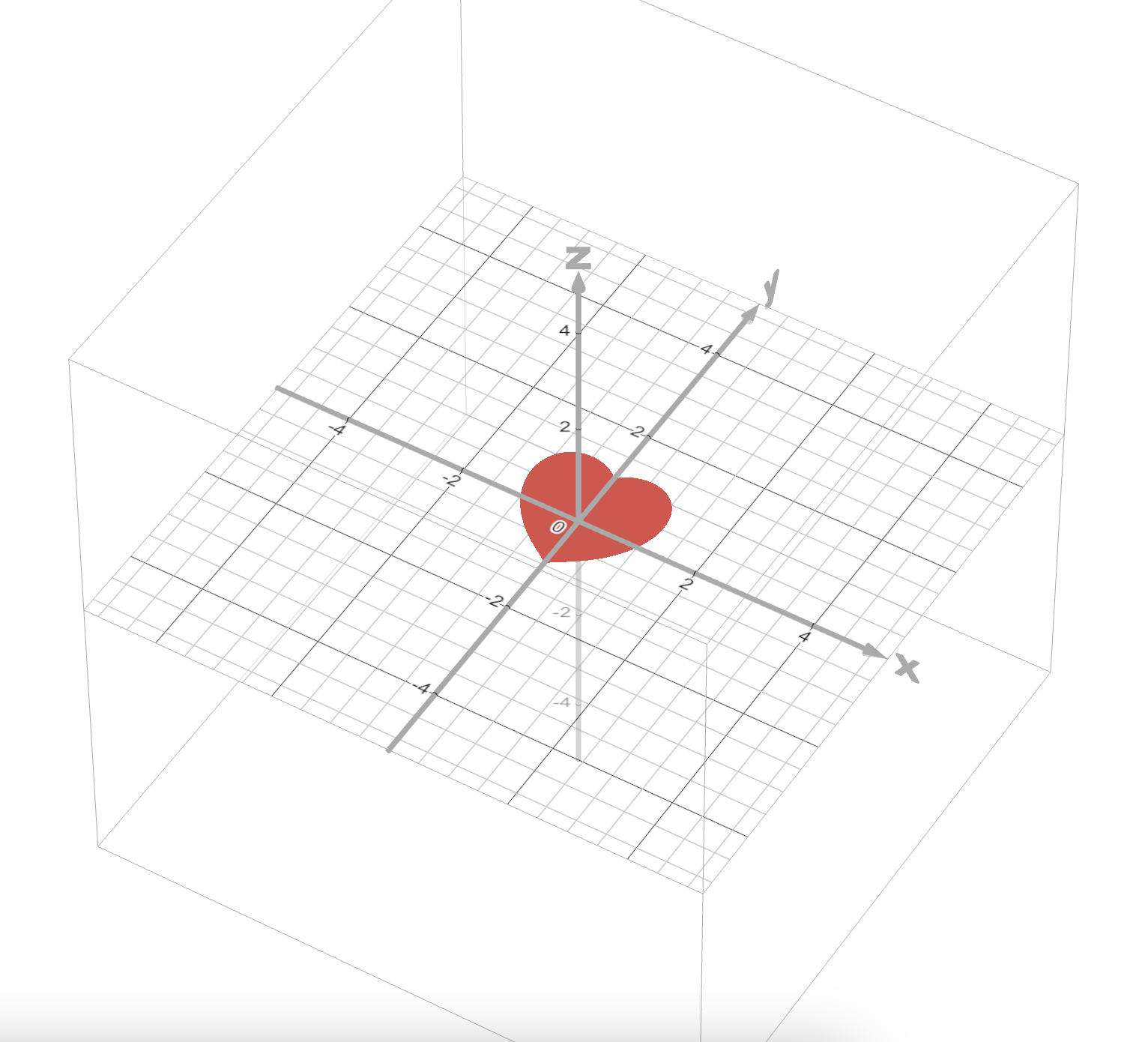
Heart curve containment (credits to Mishal Sadozai). The semialgebraic set $\{(x,y) : (x^2 + y^2 - 1)^3 \le x^2 y^3\}$, shown below, resembles a heart.

$The heart curve $\{(x,y) : (x^2 + y^2 - 1)^3 \le x^2 y^3\}$$
We prove that every point on this curve lies inside the disk of radius 2, i.e., $x^2 + y^2 \le 4$. This is a Putinar certificate over a semialgebraic set with a single degree-6 constraint. At order 3, the order-based truncation automatically gives the constraint's block a single-constant basis, while the free block gets a full degree-3 basis. The entire proof is one line:

# Python
from sos import putinar
import sympy as sp
x, y = sp.symbols('x y')
f = sp.Poly(4 - x**2 - y**2, x, y)
gs = [sp.Poly(x**2 * y**3 - (x**2 + y**2 - 1)**3, x, y)]
result = putinar(f, gs, order=3)

-- Lean
example (x y : ℝ) (h1 : (x^2+y^2-1)^3 ≤ x^2*y^3) : x^2 + y^2 ≤ 4 := by
  putinar_decomp (order := 3)

Muhammad Maaz

References

Grigoriy Blekherman, Pablo A. Parrilo, and Rekha R. Thomas (eds.), Semidefinite Optimization and Convex Algebraic Geometry, MOS-SIAM Series on Optimization, vol. 13, SIAM, Philadelphia, PA, 2012.
(PDF; doi:10.1137/1.9781611972290)
David Hilbert, Ueber die Darstellung definiter Formen als Summe von Formenquadraten, Mathematische Annalen32 (1888), 342--350.
(link)
Emil Artin, Über die Zerlegung definiter Funktionen in Quadrate, Abhandlungen aus dem Mathematischen Seminar der Universität Hamburg5 (1927), 100--115.
(doi:10.1007/BF02952513)
Theodore S. Motzkin, The arithmetic-geometric inequality, in O. Shisha (ed.), Inequalities, Academic Press, New York, 1967, 205--224.
Pablo A. Parrilo, Semidefinite programming relaxations for semialgebraic problems, Mathematical Programming96 (2003), no. 2, 293--320.
(doi:10.1007/s10107-003-0387-5)
Michel X. Goemans and David P. Williamson, Improved approximation algorithms for maximum cut and satisfiability problems using semidefinite programming, Journal of the ACM42 (1995), no. 6, 1115--1145.
(doi:10.1145/227683.227684)
Konrad Schmudgen, The K-moment problem for compact semi-algebraic sets, Mathematische Annalen289 (1991), no. 1, 203--206.
(doi:10.1007/BF01446568)
Mihai Putinar, Positive polynomials on compact semi-algebraic sets, Indiana University Mathematics Journal42 (1993), no. 3, 969--984.
(doi:10.1512/iumj.1993.42.42045)
Helfried Peyrl and Pablo A. Parrilo, Computing sum of squares decompositions with rational coefficients, Theoretical Computer Science409 (2008), no. 2, 269--281.
(doi:10.1016/j.tcs.2008.09.025)
Erich L. Kaltofen, Bin Li, Zhengfeng Yang, and Lihong Zhi, Exact certification in global polynomial optimization via sums-of-squares of rational functions with rational coefficients, Journal of Symbolic Computation47 (2012), no. 1, 1--15.
(doi:10.1016/j.jsc.2011.08.002)
Bruce Reznick, Uniform denominators in Hilbert's seventeenth problem, Mathematische Zeitschrift220 (1995), 75--97.
(doi:10.1007/BF02572604)